Cell and receptor architecture

This exercise uses cell distribution datasets to explore and compare spatial patterns of different cell types within a brain region, either within the same species or across species. 

1. Explore: To find cell distribution datasets on the EBRAINS Knowledge Graph (https://search.kg.ebrains.eu), search for “distribution” and filter by the LocaliZoom service. You may additionally refine results by species. Follow the “View data in LocaliZoom” links to open the dataset in the viewer. 

2. Navigate and Interpret: Navigate to a region of interest to inspect cell distributions, and examine how these distributions vary across sections as you navigate through the serial images.  You can zoom into different regions and adjust the atlas opacity using the slider at the top. Note any distinctive features or spatial trends.

Serial section showing the distribution of calbindin positive neurons for subject Mouse10 from the dataset “Distribution of calbindin positive neurons in the normal adult mouse brain v1” (doi: 10.25493/KHNT-KV8). Left image shows the labelled calbindin positive neurons in the bed nuclei of the stria terminalis, while the right image shows the same section with custom annotations in LocaliView.

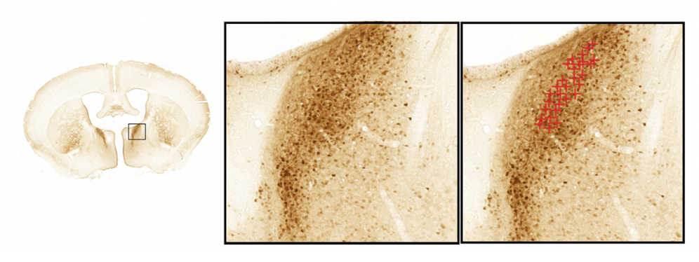
3.Annotate: Open the dataset in the LocaliView service if you wish to make your own annotations (https://localiview.apps.ebrains.eu/). You need an EBRAINS account. Create a new project and open it. Click add/edit series, and then click "Import from KG datasets", and find the relevant dataset using either the name or DOI. Click "Import this series" for the relevant image series and then click Submit. Open the series and click "Continue in LocaliZoom". You can press the space bar to annotate cells. Consult the LocaliView manual for details (https://localiview.readthedocs.io).

4. Compare: Compare observations within the dataset by tracking a region of interest across different serial sections images and examining how patterns change. You may also compare across subjects where available, using the 3D atlas as reference where needed to relate observations to anatomical structure.

This exercise demonstrates how cell distribution datasets can be used to investigate a research question by relating them to pathology markers. For example: Do amyloid-beta deposits co-localise with parvalbumin positive neurons in the adult mouse brain? 

1. Explore: Search the EBRAINS Knowledge Graph for a dataset related to your research question (e.g., amyloid-beta deposits) and filter by the LocaliZoom service. Study the histological sections by navigating across regions of interest. Identify and inspect relevant features (e.g., amyloid-beta deposits) across serial sections.
2. Select and Interpret: Select a complementary cell distribution dataset in the same species (e.g., parvalbumin positive neurons), available in MeshView through the service filters. Click View this data in MeshView to explore this dataset independently and interpret its spatial distribution across brain regions. Consider how the observed cell distribution may relate to the pathological features identified in the first dataset.
3. Compare: Annotate points of interest in the first dataset using the LocaliView service and export them as coordinates by clicking  the "MeshView JSON" button  in the top left corner. Import these into the second MeshView window by clicking "Browse" to co-visualise both datasets within a common 3D brain atlas. The imported coordinates can be made more or less visible using the slider in the right hand panel. The slider for the imported coordinates will appear at the bottom of the panel. Compare their spatial distributions to assess potential relationships (e.g., regional overlap or segregation), and reflect on how cell distribution patterns may relate to disease-associated changes.

Figure shows the distribution of parvalbumin-expressing neurons in the mouse brain (doi:10.25493/BT8X-FN9), visualized as point clouds in MeshView. Custom LocaliView annotations highlight amyloid-beta deposits (doi: 10.25493/G6CQ-D4D) overlaid on the same structures.

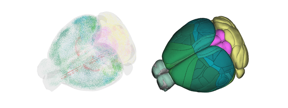
This exercise demonstrates how QUINT-derived cell distribution datasets can be used to quantify and compare neuronal populations both between individuals and across species. For example, parvalbumin-positive neurons can be explored in rat and mouse datasets to identify shared or divergent spatial patterns.

1. Explore: Search the EBRAINS Knowledge Graph and filter for the “MeshView” service to locate datasets containing QUINT point clouds. Open a dataset of interest, such as “Brain-wide quantitative data on parvalbumin positive neurons in the rat (v1),” and explore the data available for each subject.
2. Select and Analyze: Access the underlying quantification files (CSV/spreadsheet) under the “Get data” section. The number of neurons is quantified by atlas region and can be used to create plots. Use these data to examine neuron counts across regions and perform basic analyses, such as identifying areas with higher or lower parvalbumin neuron densities.
3. Visualize: Use the MeshView service link (e.g., subject_25203_pointcloud) to open the viewer. Toggle atlas meshes and brain regions on or off as needed.  Point clouds from multiple subjects can be added to the same window to compare distributions across animals. Either by uploading the JSON files using "Browse" or saving the point cloud file from one subject and uploading with it to the second Meshview window. Use this 3D visualization to interpret spatial patterns and region-specific differences in neuronal populations.
4. Go further: Analyse your own dataset with the QUINT-online workflow (https://quint-online.apps.ebrains.eu/)