Cellular architecture of the human cortex

Approximately 10 minutes · nothing to install · runs in your browser

A cytoarchitectonic map tells you where a structurally distinct brain area is. The 1 µm scans of the BigBrain show you what that structure actually looks like. In this Quick Try you select a motor area in the Julich-Brain atlas, switch to the BigBrain reference space, and zoom in until individual cell bodies become visible, among them the large Betz cells of the motor cortex. Nothing needs to be downloaded explicitly, necessary image data is streamed from the cloud while you navigate.

A) The motor area selected in the parcellation map. B) The corresponding location in BigBrain – coronal view maximized. C) Full resolution view to find individual cells.

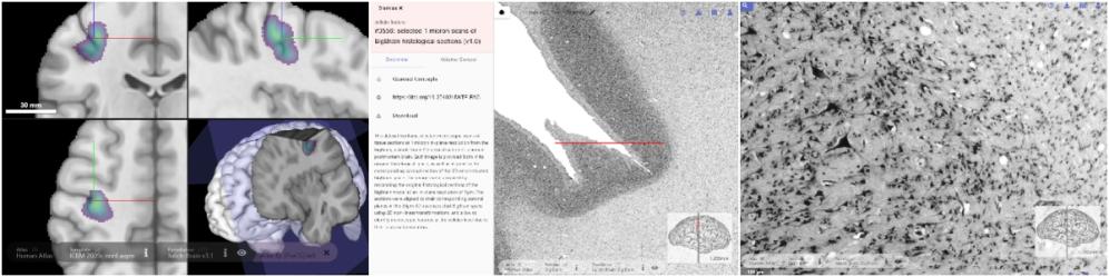
1.Explore.  Open the 3D atlas viewer siibra-explorer from the EBRAINS website under Data, Tools & Services / Brain Atlases, or directly at https://atlases.ebrains.eu/viewer. The human atlas opens in the ICBM 2009 reference space with the Julich-Brain parcellation. Click the magnifying glass in the Region Search Panel (top left), search for 4p and select Area 4p (PreCG), left hemisphere. The region sidepanel opens. Its Features tab lists the datasets anchored to this area, such as cell densities, receptor densities and connectivity.

2. Select and Interpret.  Before changing atlas template,  deselect the area 4p (as the region is not yet mapped in BigBrain) and in the Atlas Selection Panel at the bottom, switch the reference template from ICBM 2009 to BigBrain. Position and zoom are preserved: you are now looking at the corresponding piece of cortex in BigBrain.Note that siibra informs you that the region 4p left is no yet charted in this template space. Zoom into the precentral gyrus. The viewer searches the space around your current view, and the high-resolution sections (yellow lines) crossing it appear in the spatial search panel on the top left under "cellular" features (expand it if collapsed; zoom out a little if nothing shows). Pick section #3556. It loads as an overlay. Then maximize the coronal view with the square icon and keep zooming. What looked like uniform grey resolves first into laminar banding, then into individual cell bodies. In the deep layers along the anterior wall of the central sulcus, look for pyramidal cells several times larger than their neighbours: those are Betz cells, the output neurons of the primary motor cortex.

3. Compare.  Now do the same for the primary visual cortex. Leave the maximized view (icon in the bottom right). You could go back to ICBM 2009 to find it, but you don’t have to: hOc1 is mapped in BigBrain directly, so the magnifying glass will find it right where you are. Search for hOc1, select the left one to travel to its centre automatically. Deselect it, and open 1 µm sections, for example #251, near the region which would be highlighted on hover (Zoom out if the section is not present in the list, in order to see all of them). The difference is obvious without any measurement. Motor cortex is agranular: there is no distinct layer IV, and large pyramidal cells dominate. V1 shows the opposite, a dense and sharply delimited granular layer, which corresponds to the stripe of Gennari that is visible with the naked eye. Both images come from the same brain and the same staining protocol.

The same staining, two cortical types: Regions of interest in the motor (left) and visual cortex (right).

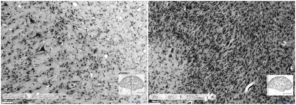
This is the workflow shown in Figure 2 of the siibra paper (Dickscheid et al., Nature Methods 2026): from a cytoarchitectonic map of area 4p, across reference spaces with the location preserved, into a 1 µm scan, down to the Betz cells in layer V. 

What you used is a sample, not a volume: 145 sections scanned at 1 µm, roughly one every millimeter through the whole brain https://doi.org/10.25493/JWTF-PAB. Next, a closer look shows how to turn these observations into measurements: where a patch was taken, how thick the cortex is at that position, and which layer a given cell belongs to.

Approximately 30 minutes · Python · runs in the EBRAINS Lab, nothing to install locally

In the Quick Try you saw that motor and visual cortex are laminated differently. Here you extract underlying data programmatically using siibra-python. You let siibra sample a cortical image patch for you, and read the corresponding layer boundaries from the BigBrain cortical layer map by Wagstyl et al., providing layer thickness estimates in millimetres at a defined position, in a named brain area. Don’t be afraid: The Python code needed to do this is short and simple!

Getting set up. The EBRAINS Lab gives you a ready-made Jupyter environment in the browser. You need a free EBRAINS account https://ebrains.eu/register; registration takes a few minutes. Then open https://lab.ebrains.eu, start a server, create a Python notebook and run !pip install siibra in the first cell. The same notebook runs unchanged in Google Colab.

A) Image patch chosen by siibra. B) Layer surfaces projected onto the image patch. C) Cortical profile defined by the projected layer surfaces.

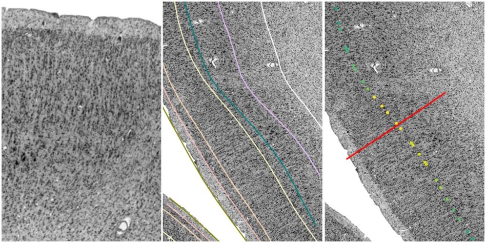
1 · Explore.  Let siibra extract a cortical image patch for you instead of downloading a large image: You tell siibra to use the probabilistic map of a brain area and get back cortical image patches at 1 µm — centred on the cortex, spanning its full thickness, sorted by how strongly the map speaks for that location:

import numpy as np
import matplotlib.pyplot as plt
import siibra
 
region  = siibra.get_region("julich 3.0.3", "4p left")
pmap    = region.get_regional_map("mni152", "statistical")
patches = siibra.features.get(pmap, "BigBrain1MicronPatch", lower_threshold=0.5)
print(f"{len(patches)} patches")
 
patch = patches[0]                      # highest relevance
print(f"relevance: {patch.relevance}")
print(f"section {patch.bigbrain_section}")
img   = patch.fetch()                   # 1 µm, upright, full cortical thickness
plt.imshow(img.get_fdata().squeeze(), cmap='gray')

Behind that one call, siibra intersects the cortical layer surfaces with the available 1 µm sections, scores the resulting mid-cortex points against your map, and cuts an oriented window along the cortical profile. The next section, Deep Dive, takes the machinery apart; here it is enough that the patch is anatomically defined rather than hand-picked.

2 · Select and Interpret.  Every patch carries its cortical profile: seven corresponding points on the BigBrain layer surfaces (https://doi.org/10.1371/journal.pbio.3000678), running from the pial surface to the grey/white boundary. The distances between consecutive points reflect layer thickness estimates at that location:

LAYERS = ["I", "II", "III", "IV", "V", "VI"]
 
def layer_thickness(p):
    xyz = p.profile.coordinates                            # pia → grey/white
    return np.linalg.norm(np.diff(xyz, axis=0), axis=1)    # mm, one per layer
 
t = layer_thickness(patch)
print(dict(zip(LAYERS, t.round(2))), "· total", round(t.sum(), 2), "mm")

The same numbers place the boundaries in the image. siibra samples the patch upright along the profile, so cortical depth is simply the vertical axis:

bounds = np.r_[0, np.cumsum(t)] / t.sum()      # 0 = pia, 1 = white matter
rows   = (bounds * img.shape[0]).astype(int)   # → draw as horizontal lines

Now compare the lines with the tissue underneath them critically. The layer surfaces are a whole-brain model: globally plausible, but locally not always precise. At 1 µm you can see this effect: a boundary may sit a little inside or outside the layer it is meant to delimit. For a study making claims at cellular resolution, the boundaries should be inspected and adjusted for the cortical patch if needed.

3 · Compare.  One patch is one measurement. The query in step 1 returned many, and their profiles are already in memory. Calculating a distribution is thus easy:

import pandas as pd
 
def thickness_table(spec, n=50):
    r  = siibra.get_region("julich 3.0.3", spec)
    ps = siibra.features.get(r.get_regional_map("mni152", "statistical"),
                             "BigBrain1MicronPatch", lower_threshold=0.5)
    return pd.DataFrame([layer_thickness(p) for p in ps[:n]], columns=LAYERS)
 
m1, v1 = thickness_table("4p left"), thickness_table("hoc1 left")
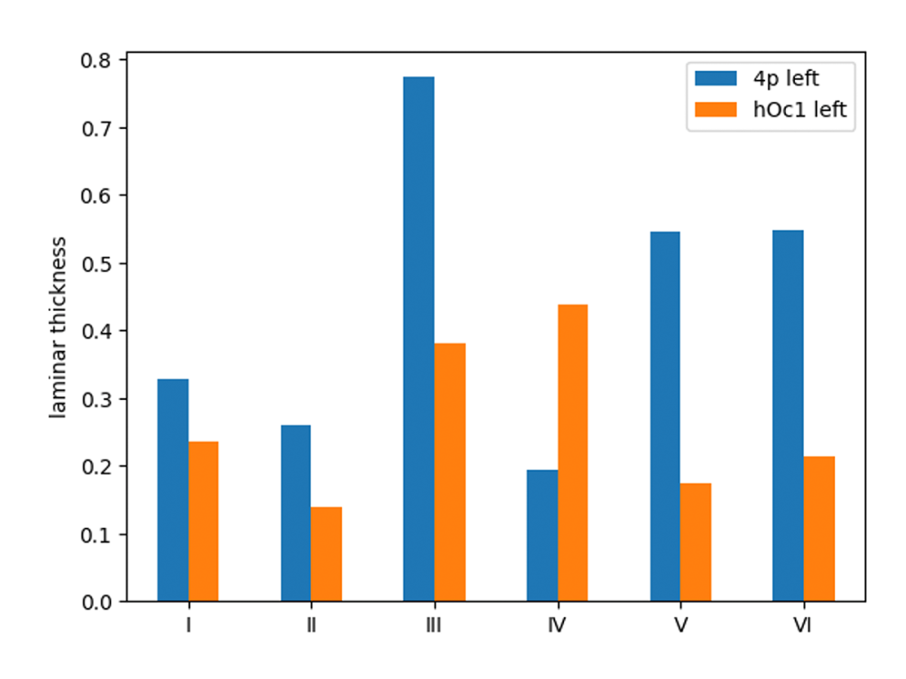
pd.concat({"4p": m1.mean(), "hOc1": v1.mean()}, axis=1).plot.bar()

This turns the impression from the Quick Try into a quantitative profile. Motor cortex is thick, and most of that thickness lies in the deep layers. V1 is thin, and a large share of it is layer IV. This is the laminar divergence between sensory and motor cortex described by Wagstyl et al., reproduced here on your own sample. 

Laminar thickness in motor and visual cortex, measured on 50 sampled patches each.

So far you have measured geometry. The content of the layers, that is how many cells there are, how large they are and how densely they are packed, is available for twelve areas as curated cell-body segmentations. Deep Dive section puts these next to receptor densities, gene expression and connectivity for the same two areas.

Approximately half a day · Python · siibra ≥ 1.0.1 and an EBRAINS account

The previous levels looked at one level of description: cells and layers in a histological section. A cytoarchitectonic area is also characterised by its receptor architecture, its gene expression and its connectivity, and in the Multilevel Human Brain Atlas all of these are accessible through the same interface. Here you query a single brain area across modalities, read the result as a multimodal signature, and compare the two areas used in the previous levels.

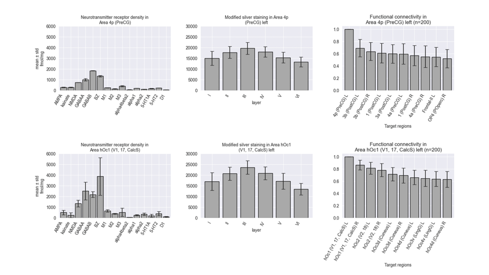
1 · Explore.  All modalities are accessed in the same way: a brain region goes in, a list of features comes out. Querying them together is a quick way to see what the atlas holds for a given area:

import siibra
 
region = siibra.get_region("julich 3.0.3", "4p left")
feature_types = [
    "LayerwiseBigBrainIntensities",
    "LayerwiseCellDensity",
    "ReceptorDensityFingerprint",
    "ReceptorDensityProfile",
    "StreamlineCounts",
    "FunctionalConnectivity"
]
for ftype in feature_types:
    print(f"{ftype:30s} {len(siibra.features.get(region, ftype))}")

Note the zeros in the output. Coverage in an atlas built from real experiments is uneven: modalities are available where they were measured, not everywhere. Area 4p has receptor densities but no segmented cell-body densities, while its neighbour 4a has it the other way around. It is worth checking this before designing an analysis, and the query above takes only seconds.

2 · Inspect and Interpret.  Two of these signatures are particularly characteristic. The receptor fingerprint gives mean densities of a dozen neurotransmitter receptors, measured by quantitative in-vitro autoradiography. The laminar staining profile gives the architectonic depth structure directly from BigBrain:

fingerprint = siibra.features.get(region, "ReceptorDensityFingerprint")[0]
fingerprint.plot()
 
laminar = siibra.features.get(region, "LayerwiseBigBrainIntensities")[0]
laminar.plot()

Both describe the same tissue, and neither can be derived from the other. This is the idea behind a multilevel atlas: cytoarchitecture, receptor architecture and connectivity are complementary organisational principles, and a brain area is characterised by their spatial correspondence rather than by any single one of them.

3 · Compare.  Now compare the two areas across all levels at once: the motor cortex from the Quick Try and the primary visual cortex from Closer look.

for spec in ["4p left", "hoc1 left"]:
    r = siibra.get_region("julich 3.0.3", spec)
    siibra.features.get(r, "ReceptorDensityFingerprint")[0].plot()
    siibra.features.get(r, "LayerwiseBigBrainIntensities")[0].plot()
    conn = [
        conn for conn in siibra.features.get(r, "FunctionalConnectivity")
        if "concatenated" in conn.name
    ][0]
    conn.plot(r, max_rows=10, kind="bar")

The four descriptions are consistent with each other: a granular, receptor-rich sensory cortex connected to the visual system, and an agranular motor cortex with large output neurons and a different connectional profile. The Quick Try showed the cytoarchitectonic part of this, and the atlas provides the remaining modalities. Figure 4 of the paper shows the same comparison for Broca’s area 44 against hOc1.

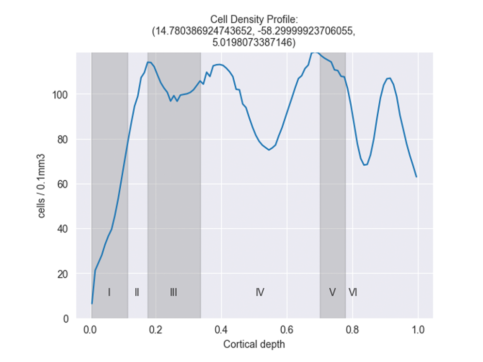
4 · Go further.  In “Closer look”, you measured laminar geometry from patches you sampled yourself. For several areas, the atlas also provides pre-processed data: every cell body segmented from 1 µm patches with a Contour Proposal Network, on manually delineated layers:

v1 = siibra.get_region("julich 3.0.3", "hoc1 left")
cd_profs = siibra.features.get(v1, siibra.features.cellular.CellDensityProfile)[0]
profile = cd_profs[-1]
# density over cortical depth
profile.plot()
# average size of individual cells per layer
profile.cells.groupby("layer")["area(micron**2)"].mean()

Comparing this with the thickness profile you measured for hOc1 in Closer look, the two observations agree: the granular layer that dominates the geometry is also where the cell counts peak, while the deeper layers contain fewer but larger cells. For the motor cortex, corresponding data are available for the neighbouring area 4a.

The atlas extends in both directions from here: down to the 1 µm patches sampled in Closer look, and up to whole-brain connectivity, gene expression and functional modes. In all cases the query is a brain region, and siibra resolves the coordinate systems in the background.