Neural connectivity

The EBRAINS Knowledge Graph provides access to many atlas integrated tract-tracing images suitable for exploration using a virtual microscopy viewer. Observations of interest can be annotated with point coordinates that can be exported for comparing observations across experiments in a 3D viewer tool.

Coronal image of a rat brain section with an anterograde tracer injection placed in the posterior area of the parietal association cortex (1), with clusters of labelled axonal fibers visible in the posterior thalamic nucleus (2). The image has id 12877_PtP_BDA_s153 and is taken from the dataset “Anterogradely labeled axonal projections from the posterior parietal cortex in rat (v1)” (doi: 10.25493/FKM4-ZCC). Scale bars, 1 mm and 500 μm (panels 1 and 2).

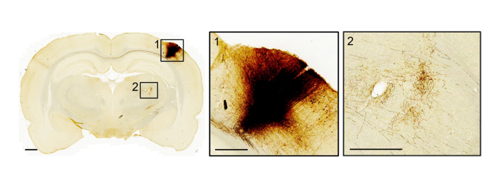
1. Explore: Find tract-tracing datasets with images in the EBRAINS Knowledge Graph (https://search.kg.ebrains.eu) using Free text search or Filters for Experimental approach “Neural connectivity”. Add other filters to fine-tune selection for species or regions of interest. Use Services filter “LocaliZoom” to identify datasets with service links “View data in LocaliZoom”, launching a viewer for navigating section images, inspecting tracer-injection sites and observing trajectories of labelled axons and their distribution within target regions across the brain.
2. Select and Interpret: Review the data descriptor documents (found in the dataset window) to find overview figures or descriptions of injection site locations. This is necessary for interpreting your observations. Relevant questions can be: What are the main brain regions connected to this injection site? Is the labelling concentrated to certain subregions or more loosely organized across a larger region? How does the pattern of labelling compare to labeling from injection sites placed in adjacent locations?
3. Compare: To compare observations across subjects, open LocaliZoom links from two data sets (preferably with similar section plane orientations) in different browsers, and navigate to corresponding locations using atlas annotations as reference. For more direct comparisons across several experiments or across datasets with different section plane orientations, annotate points of interest and export point coordinates for visualisation and comparison in a 3D atlas viewer tool (open the dataset in LocaliView; https://localiview.apps.ebrains.eu/)
4. Go further: Information about analyses performed by the data contributors can often be found in Related Resources and Publications. If you want to dive into connections for this particular set of data, refer to this dataset for an overview. Here you find overview tables from “Get Data”, containing detailed information about connections in the rat brain.

EBRAINS holds a collection of point data representing the spatial distributions of corticopontine projections identified by injection of anterograde tracers in different locations of the cerebral cortex, with the location of labelling observed within the pontine nuclei in the brain stem represented by data points integrated in the Waxholm Space rat brain atlas. The point data are configured for analysis of 3D topographical organization patterns using your own combinations of data.

Example image from the MeshView tool showing data points representing rat brain corticopontine tract tracing data from three subjects pasted into the viewer and assigned different colours. The atlas region “pontine nuclei” is rendered transparent grey, while all other atlas regions are invisible. Here, the topographical distribution in the pontine nuclei from four anterograde injections in the neocortex in rats are shown (white circled, red injection sites 12 and 13; red circled, black injection site 20 and green injection site 21). EBRAINS dataset: Leergaard, T. B., Van Swieten, M. M. H., Puchades, M. A., & Bjaalie, J. G. (2024). Topography of the complete corticopontine projection (v3) [Data set]. EBRAINS. https://doi.org/10.25493/9TMN-64U.

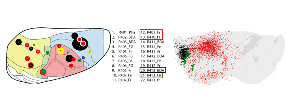
1. Explore: Find tract-tracing datasets with images in the EBRAINS Knowledge Graph using Filters for Experimental approach “Neural connectivity”, Species “Rattus norwegicus” and Services filter “MeshView” . The data sets will have service links “View data in MeshView”, launching a 3D viewer in which point data can be viewed interactively in 3D.
2. Select:  Review the data descriptor documents to find overview figures or descriptions of injection site locations. Use the description to find identifier numbers for experiments of interest. Find the relevant MeshView link at the bottom of the dataset card. 
3. Interpret: In MeshView, you will see all the point clouds and atlas region in the middle window; atlas regions hierarchy on the left and animals at the right. Here you can adjust point colour and visibility. The reference atlas regions can be made visible with the slider (in this example, only the Pontine nucleus is visible). You can now rotate the MeshView model and observe the labelling pattern.
4. Compare: To compare data from different subjects use buttons in the right column. You can change the colours of the points and change the visibility. We recommend using contrasting colors to enhance visibility between the point clouds. The axonal projections from the cortex to the pontine nuclei are aggregated in specific locations that vary with the location of tracer injections in the cortex. Try different combinations of data and see if you can see interesting patterns or organizing principles.
5. Go further: Information about analyses performed by the data contributors is available in Related Resources and Publications. The topographical organization of corticopontine projections is described in this publication.

The Allen Mouse Brain Connectivity atlas holds numerous image volumes showing axonal projections labelled following small viral tracer injection in the mouse cerebral cortex (https://connectivity.brain-map.org/). EBRAINS offers a selection of 3D point data derived from these tract-tracing experiments, configured for ready-to-go analysis of 3D spatial organization patterns using your own combination of data.

The left image shows a schematic overview of the injection sites in the mouse brain cortex, seen from above. The right image shows a 3D rendering of the mouse brain, with visible labelling in the thalamus, seen from front. In this figure, the topographical distribution in the thalamus from two anterograde injections in the somatosensory cortex in mice are shown (red circled, purple, injection site 12; dark blue, injection site 17). EBRAINs dataset: Point coordinate data showing spatial distribution of corticostriatal, corticothalamic, corticocollicular, and corticopontine projections in wild type mice (v2) [Data set]. EBRAINS. https://doi.org/10.25493/GDYP-B1B.

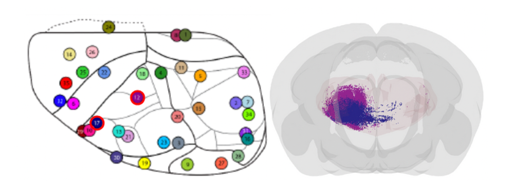
1. Explore: In EBRAINS Knowledge Graph, use Experimental approach filter “neural connectivity” and Services filter “MeshView”. This dataset provides “View data in MeshView” links. Here you can inspect point data clouds together with atlas regions visualized as meshes. The 3D viewer allows interactive 3D inspection, and possibilities to change rendering of points (visibility, size, colour). 
2. Inspect and interpret: View neural connectivity from selected cortical brain regions by opening the Data descriptor and use the injection site map to find your region of interest. To inspect specific distribution patterns you can download the shared point cloud JSON files and use a tailored version of MeshView to cut the point clouds into slices with thickness and orientation defined by you (read here for more details: https://meshview-for-brain-atlases.readthedocs.io/en/latest/displaying.html#meshview-with-double-cut-feature)
3. Define the orientation and position of the slicing by using “cut”, and change these parameters as you’d like. Choose “cloud only” if you want to only view the point cloud, and you can toggle brain regions with visibility sliders at the left side.
4. Compare: Review the data descriptor and choose injection sites from one or more experiments and download either from an individual brain region ({ExperimentNumber_BrainRegion.json}) or from all available brain regions ({ExperimentNumber_XXXX.json}) for a specific experiment. You can combine point data clouds from different data sets by downloading either multiple .json files or .txt files from “Get data” an load them in MeshView. Alternatively, you can also save a point cloud collection using the "save" button on the bottom right. A zipped folder will be created. You can upload this zipped folder in another MeshView window using the "Load" button. Refer to the MeshView manual for details ( https://meshview-for-brain-atlases.readthedocs.io).